Home Ground Advantage in AFL

So with the AFL off season underway I'm going to delve into some new stuff while there's time. I've got a few aims this off season:

• Explore some new analysis to improve upon my models for season 2020 - stuff like this HGA analysis and improving modelling of player information in match predictions.
• Explore some new modelling ideas for AFL - I'm looking into a new, more granular method of modelling AFL.
• Get an AFLW model up and running for next season.

I'm going to start off with some home ground advantage analysis. My model currently just considers travel distance and each teams historic performance at the venue to estimate the home ground advantage effect. I have a few doubts about this modelling now, such as:

• Historic venue performance is prone to over fitting. My model seems a little over fit in a few ways so I want to unwind this over fitting.
• Historic venue performance was calculated based on scoring shots, however HGA may have an impact on scoring accuracy or quality of shots generated too, so I think a score based rather than shots based model is more appropriate.
• My model was quite aggressive on the travel distance. As I don't take venue experience into consideration I think this was causing my model to weight travel distance a little too high. This meant for example that teams travelling to/from Perth were punished too much.

These doubts are based on nothing scientific, just my observations on how my models tips looked compared to other Squiggle models throughout the season.

Methodology

In this analysis, I've started with an ELO model that does not consider HGA, then I attempt to explain the margin errors using a variety of features compared for home vs away including:

• Travel Distance
• Venue Experience
• Season
• Round
• Average Historical Venue Performance
• Venue Dimensions relative to Home Venue
• Membership Figures

I found that I could explain HGA using Travel Distance + Venue Experience + Round + Average Historical Venue Performance, but all other features did not explain any of the remaining errors after these factors are taken into account. For those interested in how I came to this conclusion and how much each feature affects HGA, read on!

I started with an ELO model with no HGA considerations, so we've adjusted for team strengths as well as we can without modelling HGA. I used predictions for seasons 1897 - 2018, split into a 50% train and 50% test sets. As AFLTables designates the home team as the winner in finals, this could skew the results so I decided to exclude finals.

Next I collected the features used to explain HGA. The team specific features were calculated as differences such that a positive value should indicate an advantage to the home team. I split the values into those available for all matches, and those limited to fewer matches:

Available for all matches:

• Travel Distance: \[\log(1 + \text{Away Team Distance in km}) - \log(1 + \text{Home Team Distance in km}) \]
• Venue Experience: For the 2 seasons prior to the match (i.e. excluding the current season): \[ \frac{\text{Home Team Matches at Venue}}{\text{Home Team Matches}} - \frac{\text{Away Team Matches at Venue}}{\text{Away Team Matches}} \]
• Season: Year re based so that 1897 maps to 0 and 2018 maps to 121
• Round: \[\frac{\text{Round Number}}{\text{Total Rounds in Season}} \]
• Historical Venue Performance: Average performance at venue in terms of winning/losing margin relative to expectation in last 100 matches. I take this and multiply by matches considered/100 so there is less weight on historical venue performances over fewer matches. If a team has played less than 5 matches at the venue, I set historical venue performance to 0.

Available for select matches:

• Venue Length: \[ |\text{Away Team Venue Length} - \text{Match Venue Length}| - |\text{Home Team Venue Length} - \text{Match Venue Length}| \]
• Venue Width: \[ |\text{Away Team Venue Width} - \text{Match Venue Width}| - |\text{Home Team Venue Width} - \text{Match Venue Width}| \]
• Memberships: Based on members in prior season: \[\frac{\text{Home Team Members}}{\text{Avg Members Per Club}} - \frac{\text{Away Team Member}}{\text{Avg Members Per Club}} \]

The reasons for the transformations are as follows:

• We take the log of distance travelled as the effect is not linear. The burden of travelling from Perth to Sydney is not 22% higher than travelling from Perth to Melbourne, even though there is an extra 22% of distance to travel. Using logs puts the extra burden at 2% higher, which could still be wrong but seems more reasonable than 22%.
   
• We consider matches played at venue from the 2 prior seasons and not the current season as we don't want to introduce a feature that already has an impact from the round built in. If we use the current season, matches towards the end of the season will be assumed to have a higher HGA as there are just more matches that a team could have played at the same venue. HGA might be higher towards the end of the season, but I want to determine this by using a feature specifically for the round.
   
• We also consider venue experience as a proportion of total matches played in the 2 prior seasons. As seasons change length across the years, if we use number of matches we will be assuming HGA increases as seasons go by just due to there being more matches played in each season.
   
• We re base season so the first season is 0 so we can use a regression model with no intercept. The coefficient of the season feature will tell us how HGA has changed relative to the very first season. Using no intercept was important as I want the model to be symmetrical. I want the HGA to remain consistent regardless of the order in which teams are named. I realise there may be an increased bias in crowd support for teams named first, but I'm ignoring this for now.
   
• We express the round as a fraction relative to the total rounds in the season to again avoid any skewing of the analysis due to seasons getting longer over time. If there is a change in HGA over time, this may appear as a change in HGA by round as the high round numbers tend to only exist for very recent seasons.
   
• We've used historical venue performance from the last 100 matches as a maximum, and 5 matches as a minimum. I've also scaled the value down for small sample sizes, which is what the matches/100 does.
   
• We've calculated venue length and width measures as absolute difference from the teams' home venue. If dimensions do contribute to HGA, whether the ground is skinnier vs fatter or longer vs shorter shouldn't really matter. What should matter is that the ground dimensions are different to what the players are used to.
   
• I've expressed member figures relative to average members in that season, as membership figures have risen a lot over the years, so expressing relative to the average that year helps keep these figures distinct from the season. The membership feature also uses this value from the prior season as current season memberships are only finalised in August, so using current season values includes information about the current season which could skew the analysis.

Of these measures, travel distance and venue experience are what is commonly used to model HGA in AFL. The remainder are not normally used but I've made an attempt to investigate whether they provide any extra information in addition to travel distance and venue experience.

Analysis

As a first step, I've plotted each of the features I'm attempting to use against the model margin error to validate each makes sense and these plots can be seen below. The left plots show a scatter plot with all matches while the right shows scatter plots with the points binned into smaller intervals so we can see the trend a little easier. Note that due to sample sizes the binned plots may look strange (for example the venue performance binned plot), this is due to there being few matches in the far right bins as well as the values being out of line with the overall trend. Looking at the trend on the left is most relevant in this example.

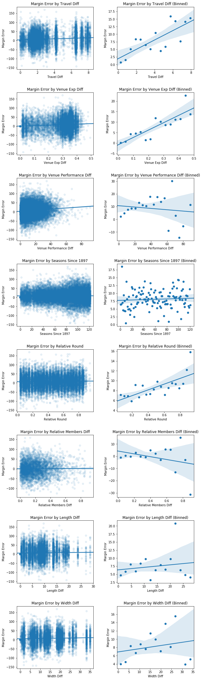
From these plots it looks like travel, venue experience, venue performance and round explain the errors the most, venue dimensions explain the errors a little and membership figures and season don't look to explain the errors much, if at all.

Now from here, I decided to first attempt to explain the errors in my ELO model using the features available for all matches. As I want to be able to model HGA back to the beginning of VFL/AFL, I want to explain HGA using features available for the entire history. After that I will attempt to use the other features to improve the HGA model further for matches where the extra features are available.

Features available in all matches are travel distance, venue experience, venue performance, season and round. To explain the model errors using these features I used forward selection linear regression. This is a method of linear regression whereby we start with no features and from the features available, add them one by one in order of which gives the biggest improvement to adjusted \(R^2\) first. We then only add more features if they improve the adjusted \(R^2\) further, and again we add the ones that give the biggest boost to the adjusted \(R^2\) first.

If we used regular \(R^2\), this would always increase as we add more features, however using adjusted \(R^2\) means we need the improvement in \(R^2\) to be more than what we would get from random chance just by adding more features. This is a good way to avoid over fitting and adding extra features just for the hell of it.

This brings us to the results, this first regression showed that we can explain the margin errors using the expression:

\[ \text{Margin Error} = 0.86 \times \text{Travel Distance} + 5.9 \times \text{Venue Experience} + 3.5 \times \text{Round} + 0.19 \times \text{Venue Performance} \]

All the coefficients here were statistically significant (p values of \( 1.5\times 10^{-6}, 3.7\times 10^{-2}, 5.2\times 10^{-3}, 4.1\times 10^{-8} \) for travel distance, venue experience, round and venue performance respectively). However using the season as a feature did not improve the adjusted \(R^2\) so was not included in the final model.

I am quite surprised that the round of the match came out as a significant factor in estimating HGA. The other features are quite easy to rationalise, but I'm at a loss for how to explain why playing a match at the end of the season at your home ground is worth about 3.5 points more than playing the match at the start of the season. Perhaps the burden of travel, the unfamiliarity and extra mental effort takes a larger toll as the season goes on and the players get more battered and bruised each week.

To see if this expression makes sense, consider what would be about the worst case scenario, West Coast or Fremantle travelling from Perth to Melbourne at the end of the season having played approx. 15% of their matches at the MCG in the prior 2 seasons while their opponent has played approx. 60% of their matches there.

According to the above expression, travelling from Perth to Melbourne is worth -7 points (distance of approx 2700km). Having played 15% of matches at the MCG relative to 60% is worth -2.5 points. And playing away from home at the end of the season relative to the start of the season is worth -3.5 points. Ignoring historical venue performance, this adds up to about a 13 point disadvantage which seems pretty reasonable to me.

Using this regression model we can then define a base HGA for each match based on travel distance, venue experience, round and venue performance. If we subtract this from our original margin error we get a new margin error which has the error from travel distance, venue experience and round built in.

As a check, the MAE for our original margin error was 27.6 points and 26.5 points after adjusting for HGA, so our adjusted margin errors have improved by about 1.1 point using these adjustments.

Next we try and explain the adjusted margin errors using venue dimensions and membership figures.

Running the forward regression model again on these 3 features, the result is that only the venue width feature was chosen to be an explanatory variable, and it had a p value of 0.025. The coefficient here was actually -0.12 as well, indicating that when a team plays at a venue which has a width different to their home venue, they actually perform better than expected.

With the coefficient being the opposite sign to what we expect and the p value not being super convincing, this is enough for me to exclude venue width as an explanatory variable, leaving none of the venue dimensions or membership figures as useful in explaining home ground advantage, after we account for venue experience, travel distance and round.

Note that above when we plotted the margin errors against the venue length and width features, we saw the expected relationship between the errors and these features. However after accounting for travel, venue experience, venue performance and round, the venue dimension features don't provide any useful extra information. As venue experience, travel distance, round and venue performance can be calculated for every match and are simpler to maintain and calculate going forwards, I am comfortable using them as a proxy for all home ground advantage factors, including venue dimensions and leaving out any specific adjustment for the actual venue dimensions.

Given the relationship between the margin errors and the membership feature above I'm not surprised it was deemed insignificant in the forward regression. Perhaps membership numbers are too noisy themselves, or are confounded with other variables such as team strength anyway and provide little additional value in estimating HGA.

Finally, if I apply the same margin error adjustment to my test data set I end up with MAE values of 27.7 prior to adjustment and 26.8 after the adjustment, so the adjustments gives a 0.9 point improvement on the test data set, slightly less than the 1.1 point improvement on the train data set but still comparable.

Conclusion

HGA can be explained using the travel distance, venue experience, venue performance and round features explained above. The linear relationship of \( \text{HGA} = 0.86 \times \text{Travel Distance} + 5.9 \times \text{Venue Experience} + 3.5 \times \text{Round} + 0.19 \times \text{Venue Performance} \) could be used to improve the margin errors for my HGA agnostic ELO model by about 1 point.

Venue dimensions appear to correlate with teams' improved performance when playing at home, however this disappears once we account for travel distance, venue experience, venue performance and round.

Membership figures and season were found to not explain any of the home ground advantage effect.

The next step is to use this methodology in an ELO model. As ELO will update team rankings based on performance accounting for HGA, the optimal weights on each feature may actually be slightly different. I would also expect to get an improvement of more than 1 point in MAE when incorporating HGA into an ELO model due to having a better estimate of team strength when HGA adjustments are made.

Data notes

Venue dimensions taken mostly from AustralianFootball.com with a few from this Foxsports article and The Footy Almanac.

Membership figures taken from Footy Industry for 1984 - 2016 and AFL website for 2017, 2018 and 2019. Due to incomplete data I only used membership figures from 1992 onwards.

Feel free to reach out on Twitter if you'd like to see any of this data.

Powered by Froala Editor

Comments