Simulating an AFL Season

I've simulated entire seasons throughout the 2019 AFL season and have been featured on Squiggle. My model came first in ladder predictions this year which I was stoked with, so thought it was about time I wrote a post about how I go about simulating the season.

Hot vs Cold?

To start with I'm going to address the hot vs cold approach which are different ways to model future matches. They differences are below:

• Hot: As matches are simulated, the simulated results are used to update team rankings which are then used to predict future matches in the same simulation.
• Cold: Teams ratings do not update after the results, but other adjustments (such as treating team ratings as random variables) can be made to account for the increased uncertainty of team ratings for future matches.

I think both methods set out to achieve the same thing: To increase the variance in results we see for matches further in the future. This increased variability tends to make our predictions more conservative as variance tends to help worse teams and hinder the strong teams which Tony Corke does a good job of explaining here. 

I think the outcome is correct with either approach, that there is increased uncertainty in matches the further away they are. However I prefer the cold approach which I would classify my methodology under. I don't update team rankings with simulated results, however, I do model additional variance by using a flatter margin -> probability function the further away the match is.

The reasons I prefer this to the hot approach are:

• It feels wrong to update team rankings in a simulated world. Say a team is expected to win 30% of the time in some match. In our simulations, they do win (approximately) 30% of the time by design. So their current ranking is exactly consistent with the results. To then update the teams' ranking in each simulation given we know the overall results are consistent with our ranking seems like a contradiction to me.
• I've found it is way more efficient to keep team rankings constant in each match but model an increase in variance of result from a code point of view. I can run about 10k season simulations in a few minutes with my approach as I don't need to simulate all matches in each simulation number from rounds 1-22 before I can even predict matches in round 23.

Approach

To start with, my margin -> probability function can be written as \( \Phi (\frac{\mu}{\sigma}) \) where \(\mu\) is the expected margin and \(\sigma\) is the expected margin standard deviation (which is actually based on a standard deviation of each teams' score errors over the past 2 seasons) and \(\Phi\) is the cumulative normal distribution function. This comes from assuming the margin is distributed normally as described here. In this model, \(\sigma\) represents the expected standard deviation (a measure of uncertainty) in the margin prediction and higher values will give a flatter margin -> probability function. With a flatter margin -> probability function, the same margin will correspond to a lower win probability.

My methodology then considers each event that happens between now and the predicted event that could alter team rankings, and adds additional variance to the variance in the margin prediction. This means that, for example, a 20 point win in the current round maps to a higher win probability than a match in 10 rounds time if the expected margin is also 20 points.

Note: \(\text{Variance} = \text{Standard Deviation}^2 \), so I convert the expected standard deviation to a variance, add additional variance for each event, then take the square root to convert it back to a standard deviation for predicting the match.

How much variance I add for each event depends on how much I expect team rankings to change based on the outcome of each event. This expectation comes from the k value used to update team rankings after each match, which is round dependent.

For example, say I'm trying to predict a round 23 match and it is currently the very start of the season. Future events that will add variance to my margin prediction are the matches each team plays from round 1 to 22.

Now, the k value used to update ELO rankings in round 1 is about 0.6, but decays each round (for example it becomes about 0.4 at round 10). Therefore, we expect rankings to change more after a round 1 match than a round 10 match. So matches from round 1 should contribute more variance than matches from round 2 which should contribute more variance than matches from round 3 and so on. I think it is important to account for how much we expect team rankings to change in modelling additional variance in future matches, this means that towards the end of the season we're not too conservative as team rankings have settled down and are relatively stable by then.

So I sum up the k values used to update rankings for all matches between now and the match I want to predict and then multiply by a constant to convert to variance. I'll explain how the constant was fitted later on.

To understand what this does, a few charts might help. This first chart shows how an expected margin maps to a win probability for a round 20 match when predicting at different points in the season. For example, a 50 point expected win in round 20 maps to a 65% win probability at the start of the season. But after round 19, a 50 point expected win maps to about a 90% win probability.

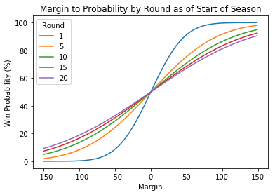
This second chart shows this mapping for different rounds at the start of the season. So if we're predicting a 25 point win at the start of the season, this corresponds to a 75% win probability for matches in round 1. However for matches in round 5 onward with an expected margin of 25 points too, this only corresponds to an approx 60% win probability.

This gives me expected scores and win probabilities for future matches, however to simulate the season I need to generate scores according to some distribution for each match so I can get a full ladder distribution including percentages.

To generate scores for each match, I assume each teams score is pulled from a gamma distribution where the mean = expected score and the variance = team variance including adjustment for how far away the match is. I then have some code to generate pairs of correlated gamma random variables (which is required as team scores are negatively correlated in AFL matches) which I can use to generate scores. The good thing about this is that to simulate 10k results for 1 match in about half a second, so I can simulate a whole season 10k times in a few minutes. Simulating finals takes a lot longer sadly as I have to run through each simulated finals series individually as each subsequent match depends on the result of the previous one.

After this I had one parameters to optimise which was the constant used to scale the k values to a variance. I fitted these by running simulations for seasons from 2001 to 2018 at different points in the season (prior to the season, round 5, round 10, round 15, round 20). I then took the predictions and scored them based on the bits measure of predicting the correct or 2 closest ladder positions.

For example, if a team finished 2nd, the score I assigned to this result was \(\text{bits}(\text{Pr(1st)} + \text{Pr(2nd)} + \text{Pr(3rd)}) \) where \(\text{bits}(x) = 1 + \log_2(x) \). I found this method OK to ensure my predictions weren't overconfident but also weren't too conservative (which they were if I didn't consider the 2 closest ladder positions).

Having discoverer rank probability score on Squiggle last year, I realised this is probably a better way to optimise things like this. Rerunning the optimisation using this measure instead gave similar results for the constant to convert k values to variances so I'm happy with the model.

Anyway, that's the nuts and bolts of my simulations methodology, hoping to tweak this to enable modelling of player information. 

Powered by Froala Editor

Comments